使用 TensorFlow 训练算法进行股票价格预测

2024年5月29日 512点热度 1人点赞 0条评论

在快速发展的金融市场中，准确的股价预测就像是圣杯。随着我们寻求更复杂的技术来解释市场趋势，机器学习成为了希望的灯塔。在各种机器学习模型中，长短期记忆 (LSTM) 网络引起了广泛关注。当与注意力机制相结合时，这些模型会变得更加强大，尤其是在分析股票价格等时间序列数据时。本文深入探讨了 LSTM 网络与 Attention 机制相结合，利用雅虎财经 ( yfinance ) 的数据预测苹果公司 ( AAPL ) 股价接下来的走势。

了解金融建模中的 LSTM 和 Attention 机制

LSTM 网络基础知识

LSTM 网络是一种循环神经网络 (RNN)，专门用于长时间记忆和处理数据序列。LSTM 与传统 RNN 的不同之处在于，它们能够长时间保存信息，这得益于其独特的结构，该结构由三个门组成：输入门（ input ）、遗忘门（ forget ）和输出门（ output ）。这些门协同管理信息流，决定保留什么和丢弃什么，从而缓解梯度消失问题——这是标准 RNN 中常见的问题。

在金融市场中，这种记住和利用长期依赖关系的能力非常宝贵。例如，股票价格不仅受近期趋势的影响，还受随时间推移而形成的模式的影响。LSTM 网络能够熟练地捕捉这些时间依赖关系，使其成为金融时间序列分析的理想选择。

Attention 机制：增强 LSTM

Attention 机制最初在自然语言处理领域流行，后来逐渐进入金融等其他领域。它基于一个简单而深刻的概念：输入序列中并非所有部分都同等重要。通过允许模型专注于输入序列的特定部分而忽略其他部分，Attention 机制增强了模型的上下文理解能力。

将 Attention 机制融入 LSTM 网络可使模型更加专注和更具情境感知能力。在预测股票价格时，某些历史数据点可能比其他数据点更相关。Attention 机制使 LSTM 能够更重视这些点，从而做出更准确、更细致的预测。

财务模式预测的相关性

LSTM 与 Attention 机制的结合创建了一个稳健的金融模式预测模型。金融市场是一个复杂的自适应系统，受多种因素影响，并表现出非线性特征。传统模型往往无法捕捉这种复杂性。然而，LSTM 网络，尤其是与注意力机制结合时，擅长解开这些模式，提供对未来股票走势的更深入理解和更准确的预测。

随着我们继续构建和实施具有 Attention 机制的 LSTM 来预测 AAPL 股票的未来4天的股价走势预测，我们深入研究了复杂的金融分析领域，该领域有望帮助我们解读和应对股票市场不断变化的动态的方式。

实验过程

接下来的工作，我们使用 Google Colab 环境来进行开发和验证。

设置您的环境

要开始构建用于预测 AAPL 股票模式的 LSTM 模型，第一步是在 Google Colab 中设置我们的编码环境。Google Colab 提供基于云的服务，该服务提供带有 GPU 支持的免费 Jupyter 笔记本环境，非常适合运行深度学习模型。

!pip install tensorflow -qqq 
!pip install keras -qqq 
!pip install yfinance -qqq

安装完成后，我们可以将这些库导入到我们的Python环境中。运行以下代码：

import tensorflow as tf
import keras
import yfinance as yf
import numpy as np
import pandas as pd
import matplotlib.pyplot as plt

# Check TensorFlow version
print("TensorFlow Version: ", tf.__version__)

该代码不仅导入库，还检查 TensorFlow 版本以确保所有内容都是最新的。Google Colab 免费版本集成的是 tensorflow 2.15.0 版。

从 yfinance 获取数据

要分析 AAPL 股票模式，我们需要历史股价数据。这就是 yfinance python 包发挥作用的地方。这个库旨在从 Yahoo Finance 获取历史市场数据。

在 Colab 笔记本中运行以下代码以下载 AAPL 的历史数据：

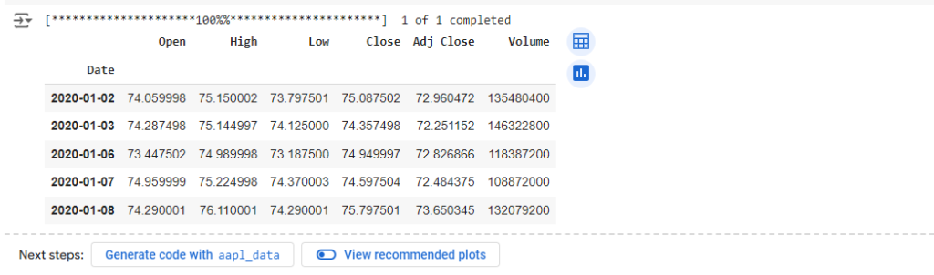
# Fetch AAPL data
aapl_data = yf.download('AAPL', start='2020-01-01', end='2024-01-01')

# Display the first few rows of the dataframe
aapl_data.head()

该脚本获取 2020 年 1 月 1 日至 2024 年 1 月 1 日期间 Apple Inc. 的每日股票价格。您可以根据自己的喜好调整开始和结束日期。

获取到的股票数据显示如下。篇幅关系，只显示了最前面的5条数据。

数据预处理和特征选择

获取数据后，预处理和特征选择变得至关重要。预处理包括清理数据并使其适合模型。这包括处理缺失值、规范化或缩放数据，以及可能创建其他特征（如移动平均值或百分比变化），这些特征可以帮助模型更有效地学习。

特征选择是指选择对预测变量贡献最大的一组正确特征。对于股票价格预测，通常使用开盘价、收盘价、最高价、最低价和成交量等特征。选择提供相关信息的特征很重要，以防止模型从噪音中学习。

在接下来的部分中，我们将预处理这些数据并构建带有注意层的 LSTM 模型来开始进行预测。

数据预处理和准备

在构建我们的 LSTM 模型之前，第一个关键步骤是准备我们的数据集。本节介绍数据预处理的基本阶段，以使来自 yfinance 的 AAPL 股票数据可用于我们的 LSTM 模型。

数据清理

股票市场数据集通常包含异常或缺失值。处理这些问题对于防止预测不准确至关重要。

识别缺失值：检查数据集中是否有缺失数据。如果有，您可以选择使用正向填充或反向填充等方法填充它们，或者完全删除这些行。

# Checking for missing values
aapl_data.isnull().sum()

# Filling missing values, if any
aapl_data.fillna(method='ffill', inplace=True)

处理异常：有时，由于数据收集过程中出现故障，数据集会包含错误值。如果发现任何异常（例如不切实际的股票价格极端飙升），则应予以纠正或删除。

特征选择

在股票市场数据中，各种特征都可能产生影响。通常使用“开盘价”、“最高价”、“最低价”、“收盘价”和“成交量”。

决定特征：对于我们的模型，我们将使用“收盘价”，但您可以尝试其他特征，如“开盘价”、“最高价”、“最低价”和“成交量”。

正常化（ Normalization ）

正常化是一种用于将数据集中数字列的值更改为通用比例的技术，而不会扭曲值范围的差异。

应用最小-最大缩放：这会缩放数据集，以便所有输入特征都位于 0 和 1 之间。

from sklearn.preprocessing import MinMaxScaler

scaler = MinMaxScaler(feature_range=(0,1))
aapl_data_scaled = scaler.fit_transform(aapl_data['Close'].values.reshape(-1,1))

创建序列

LSTM 模型要求输入为序列格式。我们将数据转换为序列，以供模型学习。

定义序列长度：选择序列长度（例如 60 天）。这意味着，对于每个样本，模型将查看过去 60 天的数据以进行预测。

X = []
y = []

for i in range(60, len(aapl_data_scaled)):
    X.append(aapl_data_scaled[i-60:i, 0])
    y.append(aapl_data_scaled[i, 0])

分割训练集和测试集

将数据分成训练集和测试集，以正确评估模型的性能。

定义分割比例：通常，80％的数据用于训练，20％用于测试。

train_size = int(len(X) * 0.8)
test_size = len(X) - train_size

X_train, X_test = X[:train_size], X[train_size:]
y_train, y_test = y[:train_size], y[train_size:]

重塑 LSTM 数据

最后，我们需要将数据重塑为[samples, time steps, features]LSTM 层所需的 3D 格式。

重塑数据：

X_train, y_train = np.array(X_train), np.array(y_train)
X_train = np.reshape(X_train, (X_train.shape[0], X_train.shape[1], 1))

在下一节中，我们将利用这些预处理的数据来构建和训练具有注意力机制的 LSTM 模型。

构建带 Attention 机制的 LSTM 模型

在本节中，我们将深入研究如何构建添加了 Attention 机制的 LSTM 模型，该模型专门用于预测 AAPL 股票模式。这需要 TensorFlow 和 Keras，它们应该已在您的 Colab 环境中设置好。

创建 LSTM 层

我们的 LSTM 模型将由几层组成，其中包括用于处理时间序列数据的 LSTM 层。基本结构如下：

from keras.models import Sequential
from keras.layers import LSTM, Dense, Dropout, AdditiveAttention, Permute, Reshape, Multiply

model = Sequential()

# Adding LSTM layers with return_sequences=True
model.add(LSTM(units=50, return_sequences=True, input_shape=(X_train.shape[1], 1)))
model.add(LSTM(units=50, return_sequences=True))

在这个模型中，units表示每个 LSTM 层中的神经元数量。return_sequences=True在第一层中至关重要，以确保输出包含序列，这对于堆叠 LSTM 层至关重要。当我们为注意层准备数据时，最后的 LSTM 层不会返回序列。

整合 Attention 机制

可以添加 Attention 机制来增强模型关注相关时间步骤的能力：

# Adding self-attention mechanism
# The attention mechanism
attention = AdditiveAttention(name='attention_weight')
# Permute and reshape for compatibility
model.add(Permute((2, 1))) 
model.add(Reshape((-1, X_train.shape[1])))
attention_result = attention([model.output, model.output])
multiply_layer = Multiply()([model.output, attention_result])
# Return to original shape
model.add(Permute((2, 1))) 
model.add(Reshape((-1, 50)))

# Adding a Flatten layer before the final Dense layer
model.add(tf.keras.layers.Flatten())

# Final Dense layer
model.add(Dense(1))

# Compile the model
# model.compile(optimizer='adam', loss='mean_squared_error')

# Train the model
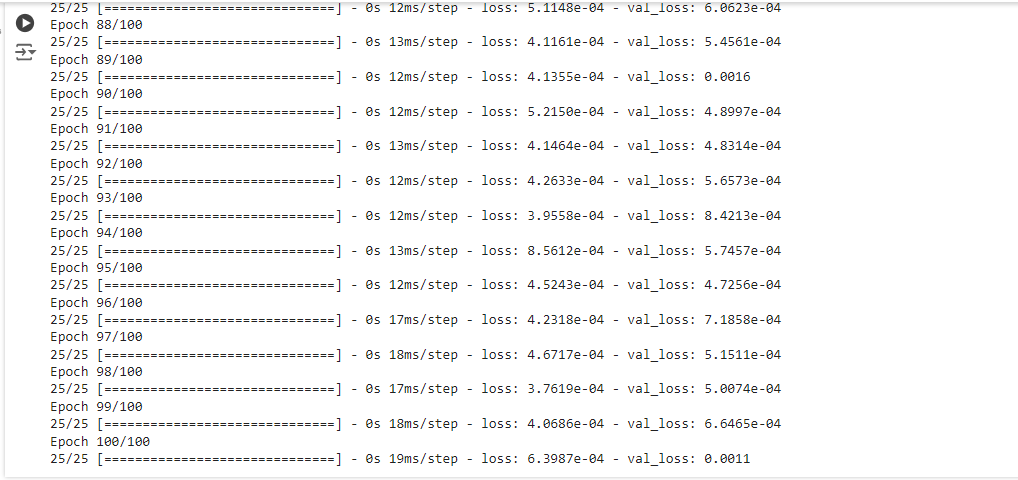
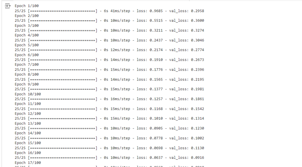
history = model.fit(X_train, y_train, epochs=100, batch_size=25, validation_split=0.2)

该自定义层计算输入序列的加权和，使模型更加关注某些时间步骤。

训练总共进行了100个 Epoch，到训练结束时，loss 值为 6.3987e-04 。

优化模型

为了增强模型的性能并降低过度拟合的风险，我们采用了 Dropout 和 Batch Normalization。

from keras.layers import BatchNormalization

# Adding Dropout and Batch Normalization
model.add(Dropout(0.2))
model.add(BatchNormalization())

在训练期间的每次更新中，Dropout 会随机将一部分输入单元设置为 0，从而有助于防止过度拟合，而批量标准化则可以稳定学习过程。

模型编译

最后，我们使用适合回归任务的优化器和损失函数来编译模型。

model.compile(optimizer='adam', loss='mean_squared_error')

adam 优化器通常是循环神经网络的一个不错的选择，而均方误差作为像我们这样的回归任务的损失函数效果很好。

模型摘要

查看模型摘要对于了解其结构和参数数量很有帮助。

model.summary()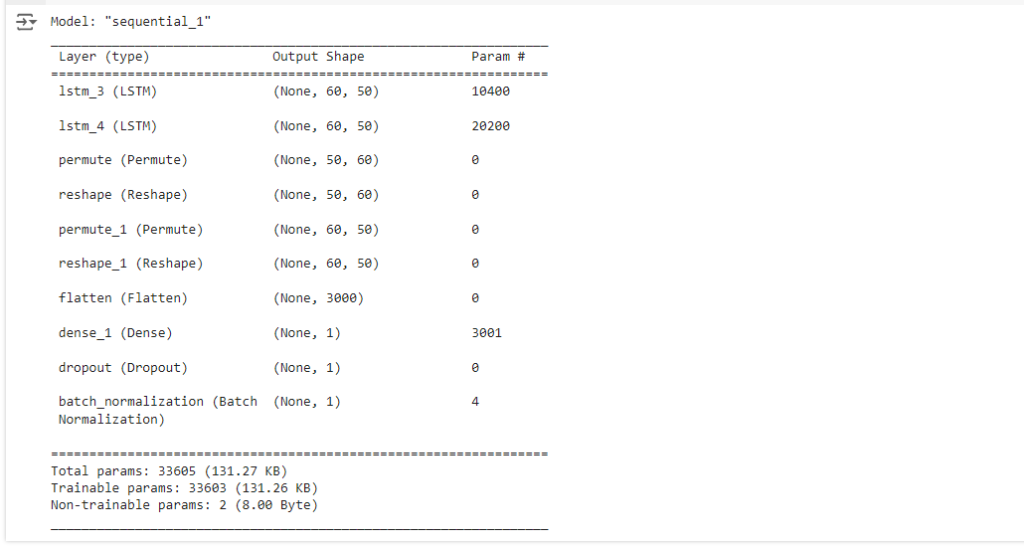

训练模型

现在，我们已构建了具有注意力机制的 LSTM 模型，接下来要使用我们准备好的训练集对其进行训练。此过程包括将训练数据输入到模型中，并让模型学习进行预测。

训练代码

使用以下代码来训练你的模型X_train：y_train

# Assuming X_train and y_train are already defined and preprocessed
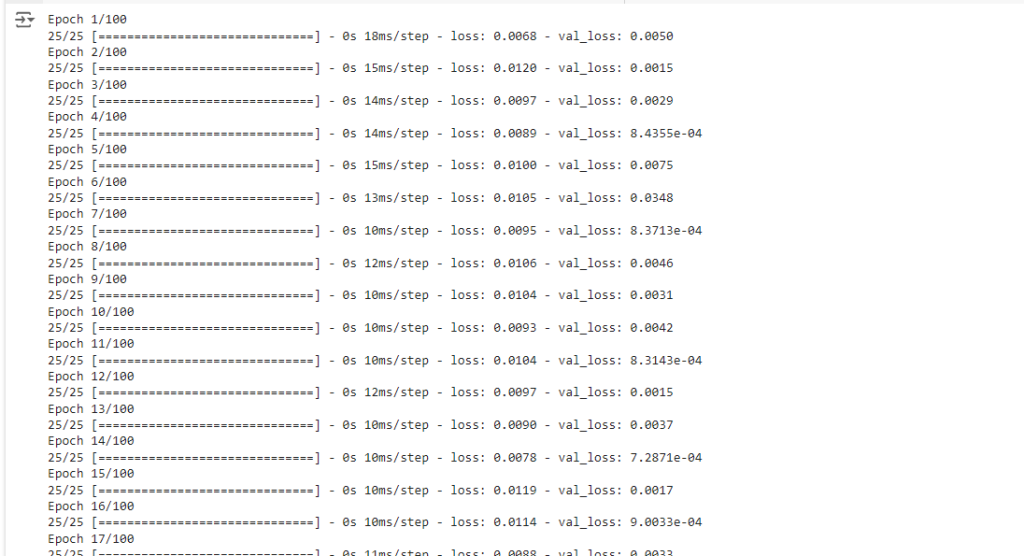
history = model.fit(X_train, y_train, epochs=100, batch_size=25, validation_split=0.2)

在这里，我们对模型进行 100 个 epoch 的训练，batch size 为 25。该validation_split参数保留了一部分训练数据用于验证，使我们能够在训练期间监控模型对未见数据的性能。

过度拟合及其避免方法

当模型学习特定于训练数据的模式，而这些模式无法推广到新数据时，就会发生过度拟合。以下是避免过度拟合的方法：

验证集：使用验证集（就像我们在训练代码中所做的那样）有助于监控模型在看不见的数据上的性能。
提前停止：当模型在验证集上的性能开始下降时，此技术会停止训练。在 Keras 中实现提前停止非常简单：

from keras.callbacks import EarlyStopping

early_stopping = EarlyStopping(monitor='val_loss', patience=10)
history = model.fit(X_train, y_train, epochs=100, batch_size=25, validation_split=0.2, callbacks=[early_stopping])

在这里，patience=10意味着如果连续 10 个时期验证损失没有改善，训练将停止。另外模型中已经包含的 Dropout 和 Batch Normalization 等技术也有助于减少过度拟合。

可选：更多的 callbacks

from keras.callbacks import ModelCheckpoint, ReduceLROnPlateau, TensorBoard, CSVLogger

# Callback to save the model periodically
model_checkpoint = ModelCheckpoint('best_model.h5', save_best_only=True, monitor='val_loss')

# Callback to reduce learning rate when a metric has stopped improving
reduce_lr = ReduceLROnPlateau(monitor='val_loss', factor=0.1, patience=5)

# Callback for TensorBoard
tensorboard = TensorBoard(log_dir='./logs')

# Callback to log details to a CSV file
csv_logger = CSVLogger('training_log.csv')

# Combining all callbacks
callbacks_list = [early_stopping, model_checkpoint, reduce_lr, tensorboard, csv_logger]

# Fit the model with the callbacks
history = model.fit(X_train, y_train, epochs=100, batch_size=25, validation_split=0.2, callbacks=callbacks_list)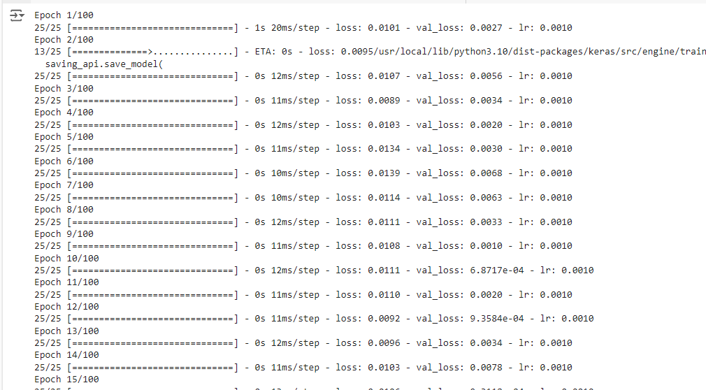

评估模型性能

训练完模型后，下一步是使用测试集评估其性能。这将让我们了解我们的模型对新的、未见过的数据的推广效果如何。

使用测试集进行评估

为了评估模型，我们首先需要以X_test与训练数据相同的方式准备测试数据（）。然后，我们可以使用模型的evaluate函数：

# Convert X_test and y_test to Numpy arrays if they are not already
X_test = np.array(X_test)
y_test = np.array(y_test)

# Ensure X_test is reshaped similarly to how X_train was reshaped
# This depends on how you preprocessed the training data
X_test = np.reshape(X_test, (X_test.shape[0], X_test.shape[1], 1))

# Now evaluate the model on the test data
test_loss = model.evaluate(X_test, y_test)
print("Test Loss: ", test_loss)

性能指标

除了损失之外，其他指标也可以提供更多关于模型性能的见解。对于像我们这样的回归任务，常见的指标包括：

平均绝对误差 (MAE)：这测量一组预测中误差的平均幅度，不考虑其方向。
均方根误差 (RMSE)：这是预测值和实际观测值之间平方差的平均值的平方根。

为了计算这些指标，我们可以使用我们的模型进行预测并将其与实际值进行比较：

from sklearn.metrics import mean_absolute_error, mean_squared_error

# Making predictions
y_pred = model.predict(X_test)

# Calculating MAE and RMSE
mae = mean_absolute_error(y_test, y_pred)
rmse = mean_squared_error(y_test, y_pred, squared=False)

print("Mean Absolute Error: ", mae)
print("Root Mean Square Error: ", rmse)

模型：

平均绝对误差（MAE）：0.0719（大约）
均方根误差 (RMSE)：0.0747（大约）

MAE 和 RMSE 都是回归模型预测准确度的度量。它们表示的内容如下：

MAE 衡量一组预测中误差的平均幅度，而不考虑其方向。它是测试样本中预测值与实际观察值之间绝对差异的平均值，其中所有个体差异具有相同的权重。MAE 为 0.0719 意味着，平均而言，模型的预测值与实际值相差约 0.0719 个单位。

RMSE 是一种二次评分规则，它还测量误差的平均幅度。它是预测值与实际观测值之间平方差的平均值的平方根。RMSE 赋予较大误差相对较高的权重。这意味着当大误差特别不受欢迎时，RMSE 应该更有用。0.0747 的 RMSE 意味着，当较大的误差受到更多惩罚时，模型的预测值平均与实际值相差 0.0747 个单位。

这些指标将帮助您了解模型的准确性以及需要改进的地方。通过分析这些指标，您可以做出明智的决定，进一步调整模型或更改方法。

在下一节中，我们将讨论如何使用该模型进行实际的股票模式预测，以及在实际应用中部署该模型的实际考虑。

预测接下来的 4 天价格

在使用注意力机制训练和评估我们的 LSTM 模型后，最后一步是利用它来预测 AAPL 股票价格的未来 4 天。

做出预测

为了预测未来的股票价格，我们需要为模型提供最新的数据点。假设我们准备了最新3个月的数据，格式如下X_train：我们想要预测第二天的价格：

import yfinance as yf
import numpy as np
from sklearn.preprocessing import MinMaxScaler

# Fetching the latest 60 days of AAPL stock data
data = yf.download('AAPL', period='3mo', interval='1d')

# Selecting the 'Close' price and converting to numpy array
closing_prices = data['Close'].values

# Scaling the data
scaler = MinMaxScaler(feature_range=(0,1))
scaled_data = scaler.fit_transform(closing_prices.reshape(-1,1))

# Since we need the last 60 days to predict the next day, we reshape the data accordingly
X_latest = np.array([scaled_data[-60:].reshape(60)])

# Reshaping the data for the model (adding batch dimension)
X_latest = np.reshape(X_latest, (X_latest.shape[0], X_latest.shape[1], 1))

# Making predictions for the next 4 candles
predicted_stock_price = model.predict(X_latest)
predicted_stock_price = scaler.inverse_transform(predicted_stock_price)

print("Predicted Stock Prices for the next 4 days: ", predicted_stock_price)

接下来我们预测未来 4 天的价格：

import yfinance as yf
import numpy as np
from sklearn.preprocessing import MinMaxScaler

# Fetch the latest 60 days of AAPL stock data
data = yf.download('AAPL', period='3mo', interval='1d')

# Select 'Close' price and scale it
closing_prices = data['Close'].values.reshape(-1, 1)
scaler = MinMaxScaler(feature_range=(0, 1))
scaled_data = scaler.fit_transform(closing_prices)

# Predict the next 4 days iteratively
predicted_prices = []
current_batch = scaled_data[-60:].reshape(1, 60, 1)  # Most recent 60 days

for i in range(4):  # Predicting 4 days
    # Get the prediction (next day)
    next_prediction = model.predict(current_batch)
    
    # Reshape the prediction to fit the batch dimension
    next_prediction_reshaped = next_prediction.reshape(1, 1, 1)
    
    # Append the prediction to the batch used for predicting
    current_batch = np.append(current_batch[:, 1:, :], next_prediction_reshaped, axis=1)
    
    # Inverse transform the prediction to the original price scale
    predicted_prices.append(scaler.inverse_transform(next_prediction)[0, 0])

print("Predicted Stock Prices for the next 4 days: ", predicted_prices)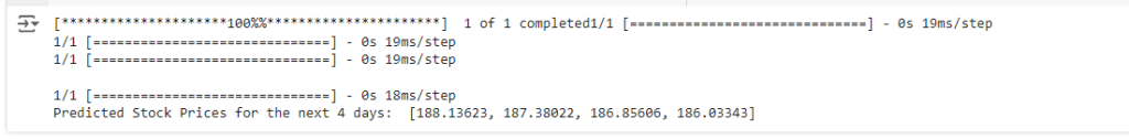

预测结果可视化

将预测值与实际股价进行直观的比较可以得到很多启发。以下是将预测股价与实际数据进行绘图的代码：

!pip install mplfinance -qqq

import pandas as pd
import mplfinance as mpf
import matplotlib.dates as mpl_dates
import matplotlib.pyplot as plt

# Assuming 'data' is your DataFrame with the fetched AAPL stock data
# Make sure it contains Open, High, Low, Close, and Volume columns

# Creating a list of dates for the predictions
last_date = data.index[-1]
next_day = last_date + pd.Timedelta(days=1)
prediction_dates = pd.date_range(start=next_day, periods=4)

# Assuming 'predicted_prices' is your list of predicted prices for the next 4 days
predictions_df = pd.DataFrame(index=prediction_dates, data=predicted_prices, columns=['Close'])

# Plotting the actual data with mplfinance
mpf.plot(data, type='candle', style='charles', volume=True)

# Overlaying the predicted data
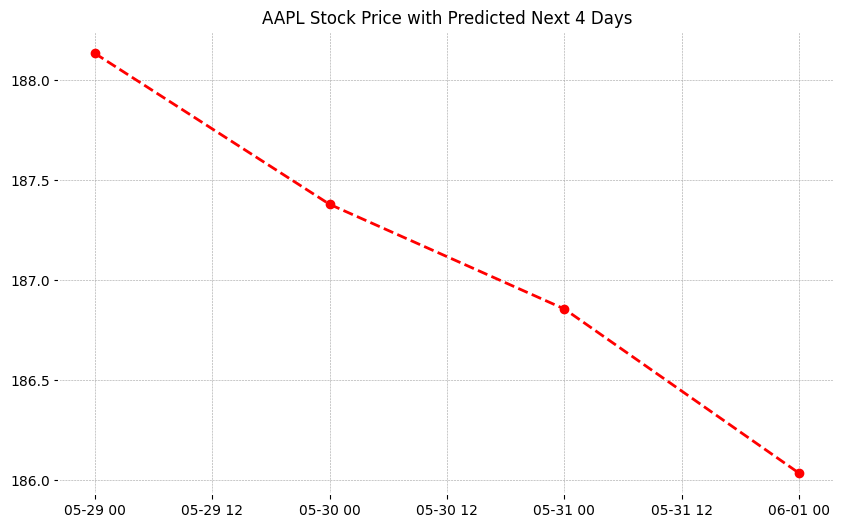
plt.figure(figsize=(10,6))
plt.plot(predictions_df.index, predictions_df['Close'], linestyle='dashed', marker='o', color='red')

plt.title("AAPL Stock Price with Predicted Next 4 Days")
plt.show()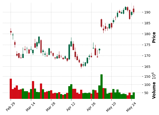

预测的视觉效果：

使用如下代码实现最终视觉效果。

import pandas as pd
import mplfinance as mpf
import matplotlib.dates as mpl_dates
import matplotlib.pyplot as plt

# Fetch the latest 60 days of AAPL stock data
data = yf.download('AAPL', period='64d', interval='1d') # Fetch 64 days to display last 60 days in the chart

# Select 'Close' price and scale it
closing_prices = data['Close'].values.reshape(-1, 1)
scaler = MinMaxScaler(feature_range=(0, 1))
scaled_data = scaler.fit_transform(closing_prices)

# Predict the next 4 days iteratively
predicted_prices = []
current_batch = scaled_data[-60:].reshape(1, 60, 1)  # Most recent 60 days

for i in range(4):  # Predicting 4 days
    next_prediction = model.predict(current_batch)
    next_prediction_reshaped = next_prediction.reshape(1, 1, 1)
    current_batch = np.append(current_batch[:, 1:, :], next_prediction_reshaped, axis=1)
    predicted_prices.append(scaler.inverse_transform(next_prediction)[0, 0])

# Creating a list of dates for the predictions
last_date = data.index[-1]
next_day = last_date + pd.Timedelta(days=1)
prediction_dates = pd.date_range(start=next_day, periods=4)

# Adding predictions to the DataFrame
predicted_data = pd.DataFrame(index=prediction_dates, data=predicted_prices, columns=['Close'])

# Combining both actual and predicted data
combined_data = pd.concat([data['Close'], predicted_data['Close']])
combined_data = combined_data[-64:] # Last 60 days of actual data + 4 days of predictions

# Plotting the actual data
plt.figure(figsize=(10,6))
plt.plot(data.index[-60:], data['Close'][-60:], linestyle='-', marker='o', color='blue', label='Actual Data')

# Plotting the predicted data
plt.plot(prediction_dates, predicted_prices, linestyle='-', marker='o', color='red', label='Predicted Data')

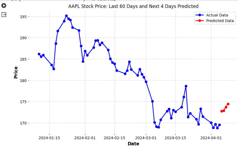
plt.title("AAPL Stock Price: Last 60 Days and Next 4 Days Predicted")
plt.xlabel('Date')
plt.ylabel('Price')
plt.legend()
plt.show()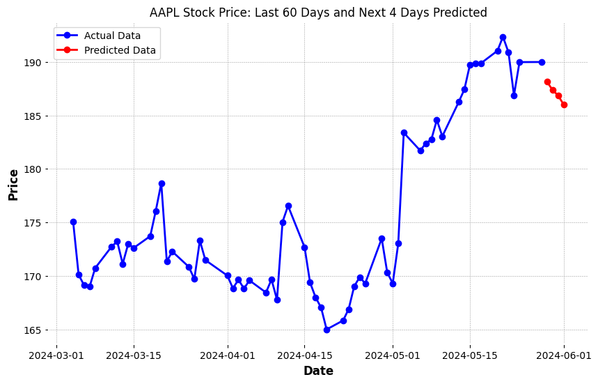

后续改进与优化

为了能达到更好的更好的训练和推理预测效果，随后又对整个方案进行了进一步的更新。更新主要包括：本地Jupyter notebook平台和GPU训练；代码重构；更多的数据样本训练算法；更长的预测时间（20天）及保存和下载预测结果到excel文件。

本地Jupyter notebook平台和GPU训练

Google Colab 虽然提供了很强大的云平台并提供免费使用的版本，但是总体来讲还是有很多资源和性能上的限制，如 Google Colab 常见问题解答里提到的：

为什么 Colab 不能保证资源供应？为了能够以较低价格动态提供大量强大的 GPU，Colab 需要保持动态调整用量限额和硬件供应情况的灵活性。
在免费版 Colab 中，用户对 GPU 等高昂资源的访问权限会受到严格限制。对于付费版 Colab，我们的目标是为用户的消费提供高价值的产品和服务。

Colab 的用量限额是多少？Colab 之所以能够免费提供资源，部分原因在于它的用量限额是时有变化的动态限额，并且它不会保证资源供应或无限供应资源。也就是说，总体用量限额、空闲超时时长、虚拟机生命周期上限、可用 GPU 类型以及其他因素都会不时变化。Colab 不会公布这些限额，原因之一是它们可能会随着时间变化。

为此我搭建了一台带GPU的机器，并安装最新的 tensorflow jupyter docker 镜像用于模型训练和推理：

docker run -it --detach --gpus all --name stock-predict -v /your_path_on_host_machine:/tf/notebooks -p 8888:8888 tensorflow/tensorflow:2.16.1-gpu-jupyter

Tensorflow 的 GPU 和 CUDA 配置一般比较容易出问题，很多时候都是因为版本不匹配的原因导致。这也是我选择使用 docker 镜像的原因，只需要在 host 端安装 GPU 驱动就可以了。具体步骤参阅 tensorflow 在线文档：https://www.tensorflow.org/install/docker 。

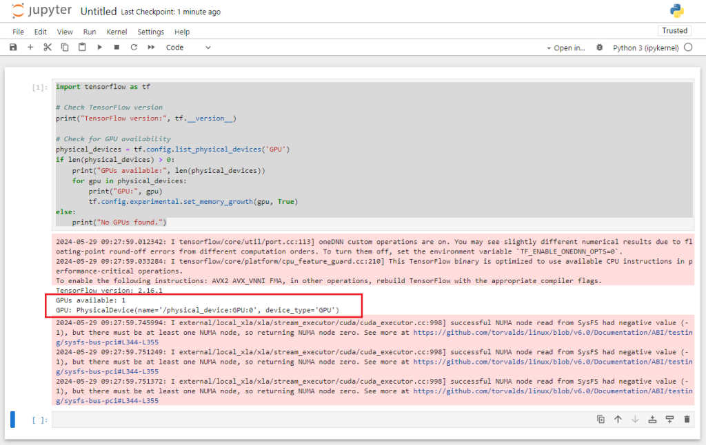
安装好后运行如下的 notebook 脚本验证 tensorflow + GPU 工作是否正常：

import tensorflow as tf

# Check TensorFlow version
print("TensorFlow version:", tf.__version__)

# Check for GPU availability
physical_devices = tf.config.list_physical_devices('GPU')
if len(physical_devices) > 0:
    print("GPUs available:", len(physical_devices))
    for gpu in physical_devices:
        print("GPU:", gpu)
        tf.config.experimental.set_memory_growth(gpu, True)
else:
    print("No GPUs found.")

出现如下的信息则表示 tensorflow 检测到了 GPU，能正常工作了。

代码重构

我们把原来 notebook 的代码进行了重构，分成了三个主要模块：历史数据获取，模型训练和股价预测。

股价历史数据获取

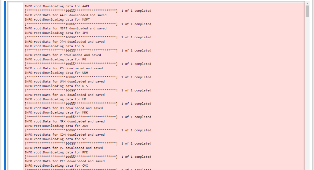
足够的股价历史数据是训练算法的基础。为此，我使用了道琼斯工业指数和纳斯达克100指数里最有代表性的公司，从雅虎财经下载这些公司20年的历史股价数据作为我们算法训练的数据集。具体收集的股票代码如下：

# Constants
DJIA_TICKERS = [
    "AAPL", "MSFT", "JPM", "V", "PG", "UNH", "DIS", "HD", "MRK", "XOM",
    "VZ", "PFE", "CVX", "KO", "NKE", "TRV", "MCD", "IBM", "BA", "MMM",
    "WBA", "GS", "AXP", "INTC", "CSCO", "JNJ", "WMT", "CAT", "RTX", "DOW"
]  # Add all DJIA tickers here
NASDAQ100_TICKERS = [
    "AAPL", "MSFT", "AMZN", "TSLA", "GOOGL", "GOOG", "NVDA", "META",
    "PEP", "ADBE", "NFLX", "PYPL", "INTC", "CMCSA", "CSCO", "AVGO",
    "TXN", "QCOM", "HON", "COST", "AMD", "SBUX", "INTU", "ISRG",
    "AMGN", "BKNG", "MDLZ", "ADI", "AMAT", "MU", "LRCX", "ASML",
    "ADP", "VRTX", "CSX", "GILD", "MRNA", "FISV", "BIIB", "MNST",
    "CHTR", "KHC", "NXPI", "ORLY", "FTNT", "MAR", "ATVI", "CTAS",
    "DLTR", "IDXX", "WBA", "WDAY", "ROST", "KLAC", "EA", "EBAY",
    "SIRI", "SNPS", "EXC", "TTWO", "CDNS", "LULU", "PAYX", "TEAM",
    "XEL", "PCAR", "FAST", "ANSS", "ILMN", "ADSK", "AEP", "CTSH",
    "CPRT", "VRSK", "OKTA", "SGEN", "WDAY", "ZS", "DDOG", "SPLK",
    "PTON", "DOCU", "CRWD", "NET", "ZM", "FANG", "REGN", "PDD",
    "JD", "NTES", "BIDU", "MELI", "MTCH", "ALGN", "CHKP", "KLAC",
    "VRSN", "CDW", "CERN", "CTXS", "MCHP", "SWKS", "TTWO", "TSLA",
    "XEL", "CSX", "DXCM", "SWKS", "REGN", "NTES", "SNPS", "VRTX"
]  # Add all NASDAQ100 tickers here

数据采集的区间则为 2004-01-01 到 2024-01-01：

STOCK_HISTORY_START_DATE = '2004-01-01'
STOCK_HISTORY_END_DATE = '2024-01-01'

下载并保存股票数据的参考代码：

def download_stock_data(tickers, start_date, end_date):
    with pd.ExcelWriter(STOCK_HISTORY_OUTPUT_FILE, engine='xlsxwriter') as writer:
        for ticker in tickers:
            logging.info(f"Downloading data for {ticker}")
            data = yf.download(ticker, start=start_date, end=end_date)
            data.to_excel(writer, sheet_name=ticker)
            logging.info(f"Data for {ticker} downloaded and saved")

具体运行效果如下：

模型训练

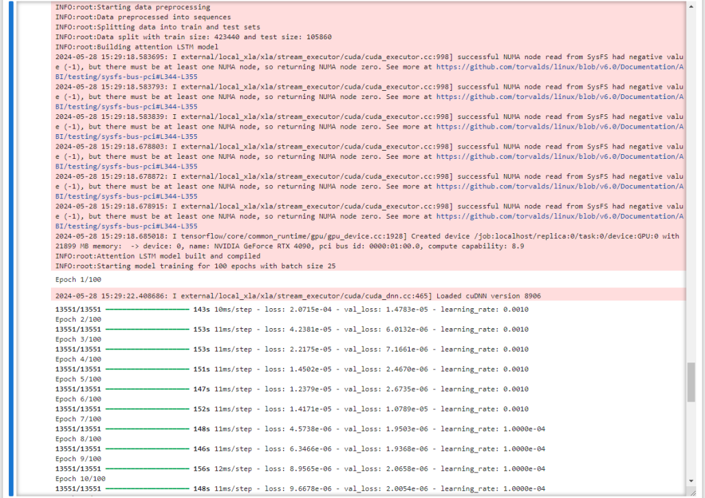
模型训练的部分则将以前的代码整合包装成两个主要的function：preprocess_data(…) 和 train_and_evaluate_model(…)。

训练部分先从保存好的股价历史数据 excel 文件中读取数据并去除无效数据（如空数据）后，使用 preprocess_data 对数据进行预处理，然后调用 train_and_evaluate_mode 对模型进行训练和评估。

    # Step 2: Load stock data for a specific ticker and preprocess
    stock_data = pd.read_excel(STOCK_HISTORY_OUTPUT_FILE, sheet_name=None)
    all_data = pd.concat(stock_data.values())
    X, y, scaler = preprocess_data(all_data, LOOKBACK_PERIOD)
    
    # Step 3: Train and evaluate model
    model, mae, rmse = train_and_evaluate_model(X, y, STOCK_PREDICT_MODEL_PATH)

运行效果如下：

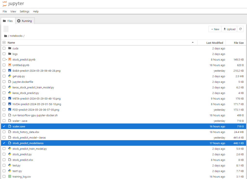
训练过程结束后，会在当前目录下生成两个文件：

股价预测

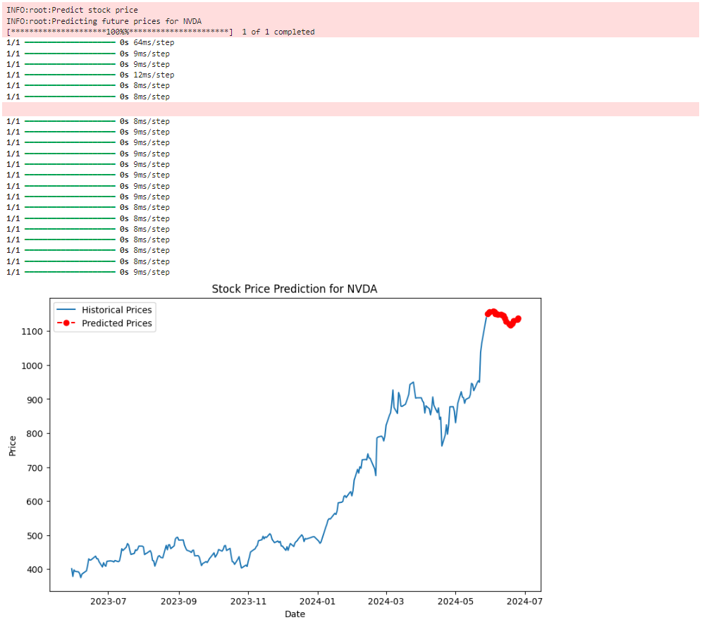
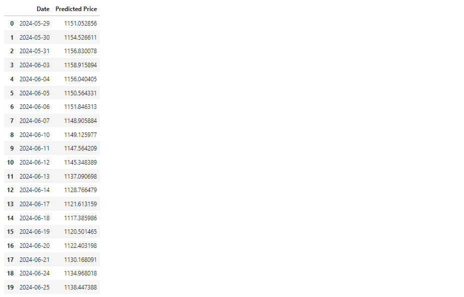
股价预测主要改进了预测的时间区间，增加预测的天数到20天，并自动跳过非交易日。另外自动保存股价预测结果到 excel 文件。参考代码如下：

PREDICTION_DAYS = 20

def predict_next_days(model, scaler, recent_data, days=PREDICTION_DAYS):

    predicted_prices = []
    current_batch = recent_data[-LOOKBACK_PERIOD:].reshape(1, LOOKBACK_PERIOD, 1)
    for _ in range(days):
        next_prediction = model.predict(current_batch)
        next_prediction_reshaped = next_prediction.reshape(1, 1, 1)
        current_batch = np.append(current_batch[:, 1:, :], next_prediction_reshaped, axis=1)
        predicted_prices.append(scaler.inverse_transform(next_prediction)[0, 0])
    return predicted_prices

def plot_predictions(ticker, data, predicted_prices):

    last_date = data.index[-1]

    # 生成只包含交易日的预测日期
    prediction_dates = []
    while len(prediction_dates) < len(predicted_prices):
        last_date += pd.Timedelta(days=1)
        if last_date.weekday() < 5:  # 跳过周末
            prediction_dates.append(last_date)

    # Creating a DataFrame to hold the prediction dates and prices
    predictions_df = pd.DataFrame({
        'Date': prediction_dates,
        'Predicted Price': predicted_prices,
        'Ticker': [ticker] * len(predicted_prices)
    })

    
    plt.figure(figsize=(10, 6))
    plt.plot(data.index, data['Close'], label='Historical Prices')
    plt.plot(predictions_df['Date'], predictions_df['Predicted Price'], linestyle='dashed', marker='o', color='red', label='Predicted Prices')
    plt.title(f"Stock Price Prediction for {ticker}")
    plt.xlabel("Date")
    plt.ylabel("Price")
    plt.legend()
    
    # Save plot to PNG file
    current_time = datetime.now().strftime("%Y-%m-%d-%H-%M-%S")
    filename = f"{ticker}-predict-{current_time}.png"
    plt.savefig(filename, format='png', dpi=300)
    
    plt.show()
    save_to_excel(predictions_df, ticker)

    display_predictions_df = pd.DataFrame({
        'Date': prediction_dates,
        'Predicted Price': predicted_prices
    })
    
    display(display_predictions_df)  # 同时以表格的形式打印日期和股价

运行效果：

结论

在本指南中，我们探索了使用带有 Attention 机制的 LSTM 网络进行股票价格预测的复杂而有趣的任务，要点包括：

LSTM 能够捕捉时间序列数据中的长期依赖关系。
Attention 机制的额外优势在于关注相关数据点。
构建、训练和评估LSTM模型的详细过程。

带有注意力机制的 LSTM 模型虽然功能强大，但也存在局限性：

假设历史模式会以类似的方式重复出现可能会带来问题，尤其是在动荡的市场中。
历史价格数据未捕捉到的市场新闻和全球事件等外部因素会显著影响股价。

浏览量: 513